|
|---|
これは日々の作業を通して学んだことや毎日の生活で気づいたことをを記録しておく備忘録である。
HTML ファイル生成日時: 2026/07/16 23:23:49.686 (台灣標準時)
SciPy を使うと、簡便に最小二乗法を利用することができるでござる。まず、 練習用のデータを生成するでござる。以下のようなスクリプトを用意して、実 行してみるでござる。
#!/usr/pkg/bin/python3.9

#
# Time-stamp: <2022/07/15 06:42:57 (CST) daisuke>
#

# importing argparse module
import argparse

# importing sys module
import sys

# importing pathlib module
import pathlib

# importing numpy
import numpy

# initialising a parser
parser = argparse.ArgumentParser (description='plotting data')

# adding arguments
parser.add_argument ('-a', '--min', type=float, default=0.0, \
                     help='minimum x value')
parser.add_argument ('-b', '--max', type=float, default=100.0, \
                     help='maximum x value')
parser.add_argument ('-s', '--slope', type=float, default=1.0, \
                     help='gradient of straight line')
parser.add_argument ('-i', '--intercept', type=float, default=0.0, \
                     help='y-intercept of straight line')
parser.add_argument ('-e', '--stddev', type=float, default=0.3, \
                     help='standard deviation of errors')
parser.add_argument ('-n', '--ndata', type=int, default=11, \
                     help='number of data points')

# parsing arguments
args = parser.parse_args ()

# input parameters
slope     = args.slope
intercept = args.intercept
x_min     = args.min
x_max     = args.max
stddev    = args.stddev
n_data    = args.ndata

# a function for straight line
def func (x, a, b):
    y = a * x + b
    return (y)

# random number generator
rng = numpy.random.default_rng ()

# generation of synthetic data
data_err = rng.normal (0.0, stddev, n_data)
data_x   = numpy.linspace (x_min, x_max, n_data)
data_y   = func (data_x, slope, intercept) + data_err

# printing generated synthetic data
for i in range ( len (data_x) ):
    print ("%8.4f %8.4f %8.4f" % (data_x[i], data_y[i], stddev) )
以下のように実行してみるでござる。
% ./gen_data.py -s 2 -i 5 -a 0 -b 45 -n 10 -e 0.3 > sample.data
% ./gen_data.py -s 2 -i 5 -a 50 -b 70 -n 5 -e 7 >> sample.data
% ./gen_data.py -s 2 -i 5 -a 75 -b 100 -n 6 -e 0.3 >> sample.data
% cat sample.data
  0.0000   5.0030   0.3000
  5.0000  14.9402   0.3000
 10.0000  25.0036   0.3000
 15.0000  35.5060   0.3000
 20.0000  44.6728   0.3000
 25.0000  55.1272   0.3000
 30.0000  65.2244   0.3000
 35.0000  74.8133   0.3000
 40.0000  84.9241   0.3000
 45.0000  94.9772   0.3000
 50.0000 108.7896   7.0000
 55.0000 121.2910   7.0000
 60.0000 116.7390   7.0000
 65.0000 137.1529   7.0000
 70.0000 139.2072   7.0000
 75.0000 154.6195   0.3000
 80.0000 164.8580   0.3000
 85.0000 175.3297   0.3000
 90.0000 185.1314   0.3000
 95.0000 194.2291   0.3000
100.0000 205.0442   0.3000
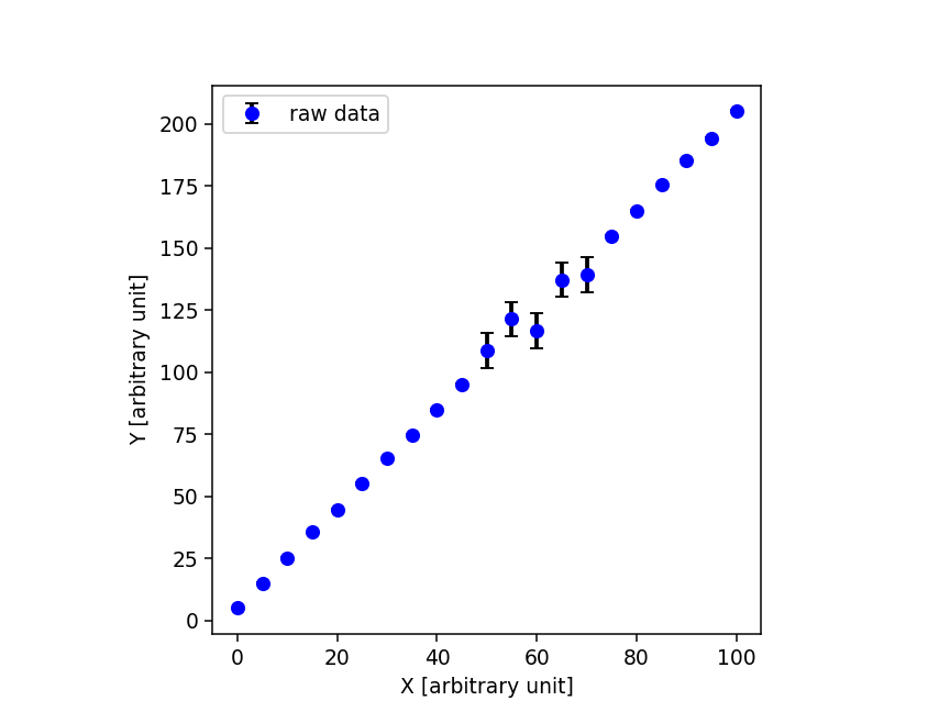
生成したデータを表示してみるでござる。
#!/usr/pkg/bin/python3.9

#
# Time-stamp: <2022/07/15 06:43:28 (CST) daisuke>
#

# importing argparse module
import argparse

# importing sys module
import sys

# importing pathlib module
import pathlib

# importing numpy module
import numpy

# importing matplotlib module
import matplotlib.figure
import matplotlib.backends.backend_agg

# initialising a parser
parser = argparse.ArgumentParser (description='plotting data')

# adding arguments
parser.add_argument ('-i', '--input', default='sample.data', \
                     help='input data file name')
parser.add_argument ('-o', '--output', default='plot.png', \
                     help='output image file name')
parser.add_argument ('-r', '--resolution', type=float, default=225, \
                     help='resolution of output image file in DPI')

# parsing arguments
args = parser.parse_args ()

# input parameters
file_input  = args.input
file_output = args.output
resolution  = args.resolution

# existence check of files
path_input  = pathlib.Path (file_input)
path_output = pathlib.Path (file_output)
if not (path_input.exists ()):
    print ("ERROR: input file '%s' does not exist." % (file_input) )
    sys.exit ()
if (path_output.exists ()):
    print ("ERROR: output file '%s' exists." % (file_output) )
    sys.exit ()
if not ( (path_output.suffix == '.eps') \
         or (path_output.suffix == '.pdf') \
         or (path_output.suffix == '.png') \
         or (path_output.suffix == '.ps') ):
    print ("ERROR: output file must be either EPS, PDF, PNG, or PS file.")
    sys.exit ()

# making empty arrays
data_x    = numpy.array ([])
data_y    = numpy.array ([])
data_yerr = numpy.array ([])

# opening input data file
with open (file_input, 'r') as fh:
    # reading file line-by-line
    for line in fh:
        # splitting a line
        (x_str, y_str, yerr_str) = line.split ()
        # converting string into float
        x    = float (x_str)
        y    = float (y_str)
        yerr = float (yerr_str)
        # appending data into arrays
        data_x    = numpy.append (data_x, x)
        data_y    = numpy.append (data_y, y)
        data_yerr = numpy.append (data_yerr, yerr)

# making objects "fig" and "ax"
fig = matplotlib.figure.Figure ()
matplotlib.backends.backend_agg.FigureCanvasAgg (fig)
ax = fig.add_subplot (111)

# axes
ax.set_xlabel ("X [arbitrary unit]")
ax.set_ylabel ("Y [arbitrary unit]")
ax.set_box_aspect (1)

# plotting data
ax.errorbar (data_x, data_y, yerr=data_yerr, marker='o', color='blue', \
             linestyle='None', ecolor='black', elinewidth=2, capsize=3, \
             label='raw data')
ax.legend ()

# saving file
fig.savefig (file_output, dpi=resolution)
実行してみると、以下のような図ができるでござる。
% ./plot_data.py -i sample.data -o sample.png -r 135
% ls -l sample.*
-rw-r--r--  1 daisuke  taiwan    567 Jul 15 06:50 sample.data
-rw-r--r--  1 daisuke  taiwan  27890 Jul 15 06:50 sample.png
% feh -dF sample.png
|
|
|---|
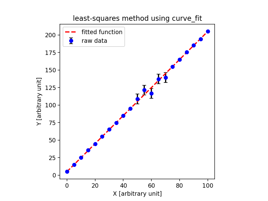
scipy.optimize.curve_fit を使って最小二乗法を行ってみるでござる。コー ドは以下の通りにござる。
#!/usr/pkg/bin/python3.9

#
# Time-stamp: <2022/07/15 06:53:39 (CST) daisuke>
#

# importing argparse module
import argparse

# importing sys module
import sys

# importing pathlib module
import pathlib

# importing numpy module
import numpy

# importing scipy
import scipy.optimize

# importing matplotlib module
import matplotlib.figure
import matplotlib.backends.backend_agg

# initialising a parser
parser = argparse.ArgumentParser (description='fitting data using curve_fit')

# adding arguments
parser.add_argument ('-i', '--input', default='sample.data', \
                     help='input file')
parser.add_argument ('-o', '--output', default='fitting.png', \
                     help='output file')
parser.add_argument ('-a', '--ainit', type=float, default=1.0, \
                     help='initial guess of a')
parser.add_argument ('-b', '--binit', type=float, default=1.0, \
                     help='initial guess of b')
parser.add_argument ('-r', '--resolution', type=float, default=225, \
                     help='resolution of output image file in DPI')

# parsing arguments
args = parser.parse_args ()

# input parameters
file_input  = args.input
file_output = args.output
a_init      = args.ainit
b_init      = args.binit
resolution  = args.resolution

# other parameters
n_data = 1000

# existence check of files
path_input  = pathlib.Path (file_input)
path_output = pathlib.Path (file_output)
if not (path_input.exists ()):
    print ("ERROR: input file '%s' does not exist." % (file_input) )
    sys.exit ()
if (path_output.exists ()):
    print ("ERROR: output file '%s' exists." % (file_output) )
    sys.exit ()
if not ( (path_output.suffix == '.eps') \
         or (path_output.suffix == '.pdf') \
         or (path_output.suffix == '.png') \
         or (path_output.suffix == '.ps') ):
    print ("ERROR: output file must be either EPS, PDF, PNG, or PS file.")
    sys.exit ()

# making empty arrays
data_x    = numpy.array ([])
data_y    = numpy.array ([])
data_yerr = numpy.array ([])

# opening input data file
with open (file_input, 'r') as fh:
    # reading file line-by-line
    for line in fh:
        # splitting a line
        (x_str, y_str, yerr_str) = line.split ()
        # converting string into float
        x    = float (x_str)
        y    = float (y_str)
        yerr = float (yerr_str)
        # appending data into arrays
        data_x    = numpy.append (data_x, x)
        data_y    = numpy.append (data_y, y)
        data_yerr = numpy.append (data_yerr, yerr)

# a function for straight line
def func (x, a, b):
    y = a * x + b
    return (y)

# initial guess of coefficients
param0 = [a_init, b_init]

# weighted least-squares fitting
# x: data_x
# y: data_y
# yerr: data_yerr
popt, pcov = scipy.optimize.curve_fit (func, data_x, data_y, p0=param0, \
                                       sigma=data_yerr)

# fitted parameters and covariance matrix
print ("popt:", popt)
print ("pcov:", pcov)

# fitted a and b
a_fitted, b_fitted = popt

# degrees of freedom
dof = len (data_x) - len (popt)
print ("dof = %d" % (dof) )

# residual and reduced chi-squared
residual     = ( data_y - func (data_x, a_fitted, b_fitted) ) / data_yerr
reduced_chi2 = (residual**2).sum () / dof
print ("reduced chi^2 = %f" % (reduced_chi2) )

# errors of a and b
a_err, b_err = numpy.sqrt ( numpy.diagonal (pcov) )
print ("a = %f +/- %f (%f %%)" % (a_fitted, a_err, a_err / a_fitted * 100.0) )
print ("b = %f +/- %f (%f %%)" % (b_fitted, b_err, b_err / b_fitted * 100.0) )

# range of data
x_min = numpy.amin (data_x)
x_max = numpy.amax (data_x)

# fitted line
fitted_x = numpy.linspace (x_min, x_max, n_data)
fitted_y = func (fitted_x, a_fitted, b_fitted)

# making objects "fig" and "ax"
fig = matplotlib.figure.Figure ()
matplotlib.backends.backend_agg.FigureCanvasAgg (fig)
ax = fig.add_subplot (111)

# axes
ax.set_title ("least-squares method using curve_fit")
ax.set_xlabel ("X [arbitrary unit]")
ax.set_ylabel ("Y [arbitrary unit]")
ax.set_box_aspect (1)

# plotting data
ax.errorbar (data_x, data_y, yerr=data_yerr, marker='o', color='blue', \
             linestyle='None', ecolor='black', elinewidth=2, capsize=3, \
             label='raw data')
ax.plot (fitted_x, fitted_y, color='red', \
         linestyle='--', linewidth=2, label='fitted function')
ax.legend ()

# saving file
fig.savefig (file_output, dpi=resolution)

|
|---|
実行結果は以下の通りにござる。 curve_fit を使うと、フィッティングによ り求まった係数の値に加えて、共分散行列も返してくれるので、便利にござる。 共分散行列の対角成分の平方根を取ればフィッティングにより求めた係数の誤 差がわかるでござる。ただ、 degrees of freedom や reduced chi-squared などは自分で計算する必要があるでござる。
% ./fit_curve_fit.py -i sample.data -o curve_fit.png -r 135
popt: [1.99776157 5.06748716]
pcov: [[ 4.42292464e-06 -2.07357894e-04]
 [-2.07357894e-04  1.47899332e-02]]
dof = 19
reduced chi^2 = 0.901579
a = 1.997762 +/- 0.002103 (0.105272 %)
b = 5.067487 +/- 0.121614 (2.399885 %)
% ls -l curve_fit.png
-rw-r--r--  1 daisuke  taiwan  41594 Jul 15 06:53 curve_fit.png
% feh -dF curve_fit.png
|
|---|
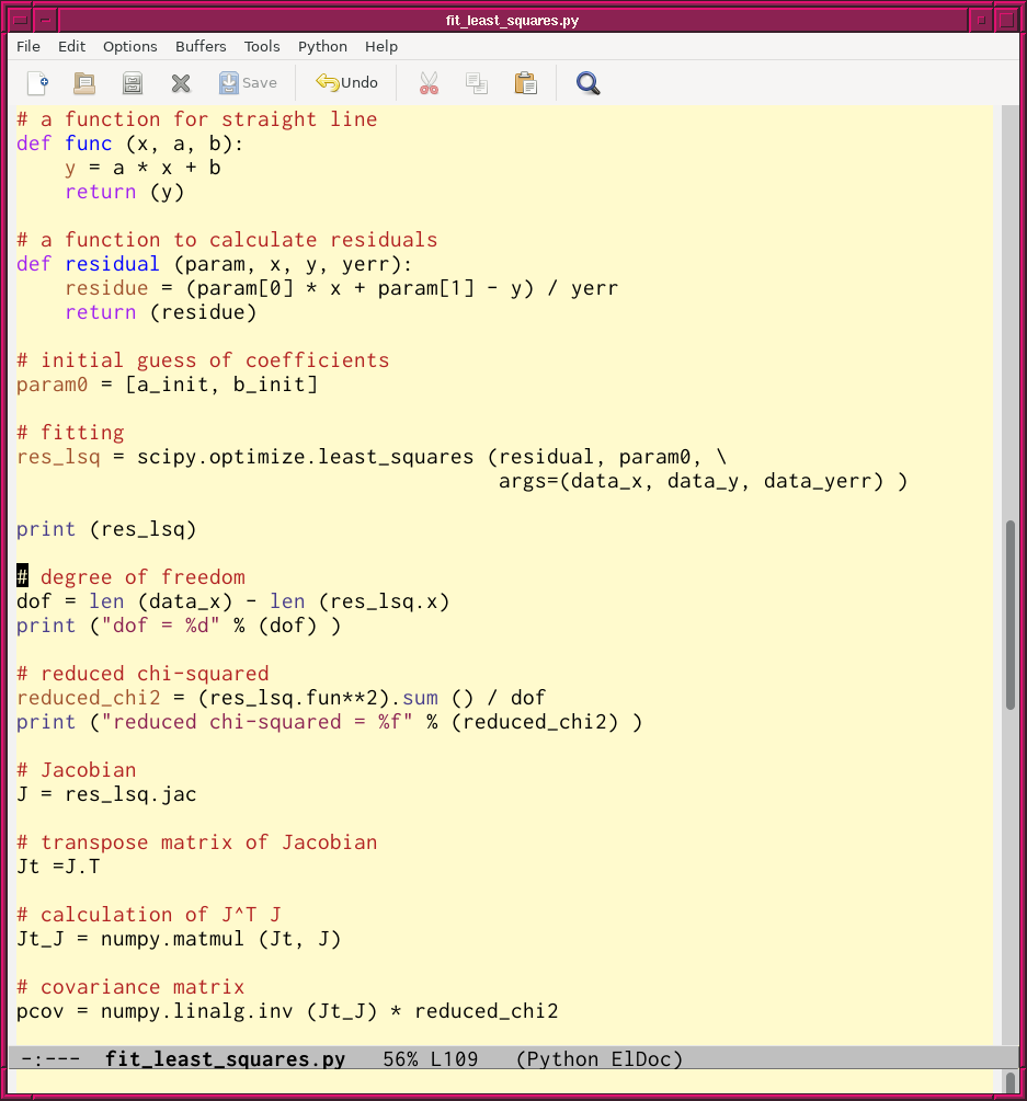
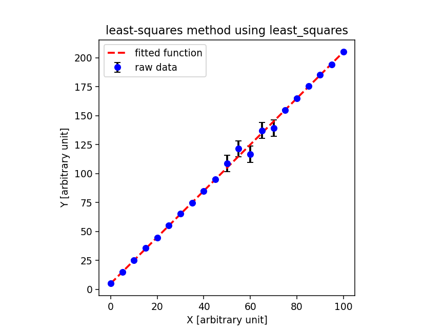
次に、 scipy.optimize.least_squares を使って最小二乗法を行ってみるでご ざる。コードは以下の通りにござる。
#!/usr/pkg/bin/python3.9

#
# Time-stamp: <2022/07/15 06:54:29 (CST) daisuke>
#

# importing argparse module
import argparse

# importing sys module
import sys

# importing pathlib module
import pathlib

# importing numpy module
import numpy

# importing scipy
import scipy.optimize

# importing matplotlib module
import matplotlib.figure
import matplotlib.backends.backend_agg

# initialising a parser
parser = argparse.ArgumentParser (description='fitting data using least_squares')

# adding arguments
parser.add_argument ('-i', '--input', default='sample.data', \
                     help='input file')
parser.add_argument ('-o', '--output', default='fitting.png', \
                     help='output file')
parser.add_argument ('-a', '--ainit', type=float, default=1.0, \
                     help='initial guess of a')
parser.add_argument ('-b', '--binit', type=float, default=1.0, \
                     help='initial guess of b')
parser.add_argument ('-r', '--resolution', type=float, default=225, \
                     help='resolution of output image file in DPI')

# parsing arguments
args = parser.parse_args ()

# input parameters
file_input  = args.input
file_output = args.output
a_init      = args.ainit
b_init      = args.binit
resolution  = args.resolution

# other parameters
n_point = 1000

# existence check of files
path_input  = pathlib.Path (file_input)
path_output = pathlib.Path (file_output)
if not (path_input.exists ()):
    print ("ERROR: input file '%s' does not exist." % (file_input) )
    sys.exit ()
if (path_output.exists ()):
    print ("ERROR: output file '%s' exists." % (file_output) )
    sys.exit ()
if not ( (path_output.suffix == '.eps') \
         or (path_output.suffix == '.pdf') \
         or (path_output.suffix == '.png') \
         or (path_output.suffix == '.ps') ):
    print ("ERROR: output file must be either EPS, PDF, PNG, or PS file.")
    sys.exit ()

# making empty arrays
data_x    = numpy.array ([])
data_y    = numpy.array ([])
data_yerr = numpy.array ([])

# opening input data file
with open (file_input, 'r') as fh:
    # reading file line-by-line
    for line in fh:
        # splitting a line
        (x_str, y_str, yerr_str) = line.split ()
        # converting string into float
        x    = float (x_str)
        y    = float (y_str)
        yerr = float (yerr_str)
        # appending data into arrays
        data_x    = numpy.append (data_x, x)
        data_y    = numpy.append (data_y, y)
        data_yerr = numpy.append (data_yerr, yerr)

# a function for straight line
def func (x, a, b):
    y = a * x + b
    return (y)

# a function to calculate residuals
def residual (param, x, y, yerr):
    residue = (param[0] * x + param[1] - y) / yerr
    return (residue)

# initial guess of coefficients
param0 = [a_init, b_init]

# fitting
res_lsq = scipy.optimize.least_squares (residual, param0, \
                                        args=(data_x, data_y, data_yerr) )

print (res_lsq)

# degree of freedom
dof = len (data_x) - len (res_lsq.x)
print ("dof = %d" % (dof) )

# reduced chi-squared
reduced_chi2 = (res_lsq.fun**2).sum () / dof
print ("reduced chi-squared = %f" % (reduced_chi2) )

# Jacobian
J = res_lsq.jac

# transpose matrix of Jacobian
Jt =J.T

# calculation of J^T J
Jt_J = numpy.matmul (Jt, J)

# covariance matrix
pcov = numpy.linalg.inv (Jt_J) * reduced_chi2

# printing covariance matrix
print ("pcov =", pcov)

# fitted a and b
a_fitted, b_fitted = res_lsq.x
a_err, b_err = numpy.sqrt ( numpy.diagonal (pcov) )
print ("a = %f +/- %f (%f %%)" % (a_fitted, a_err, a_err / a_fitted * 100.0) )
print ("b = %f +/- %f (%f %%)" % (b_fitted, b_err, b_err / b_fitted * 100.0) )

# range of data
x_min = numpy.amin (data_x)
x_max = numpy.amax (data_x)

# fitted line
fitted_x = numpy.linspace (x_min, x_max, n_point)
fitted_y = func (fitted_x, a_fitted, b_fitted)

# making objects "fig" and "ax"
fig = matplotlib.figure.Figure ()
matplotlib.backends.backend_agg.FigureCanvasAgg (fig)
ax = fig.add_subplot (111)

# axes
ax.set_title ("least-squares method using least_squares")
ax.set_xlabel ("X [arbitrary unit]")
ax.set_ylabel ("Y [arbitrary unit]")
ax.set_box_aspect (1)

# plotting data
ax.errorbar (data_x, data_y, yerr=data_yerr, marker='o', color='blue', \
             linestyle='None', ecolor='black', elinewidth=2, capsize=3, \
             label='raw data')
ax.plot (fitted_x, fitted_y, color='red', \
         linestyle='--', linewidth=2, label='fitted function')
ax.legend ()

# saving file
fig.savefig (file_output, dpi=resolution)
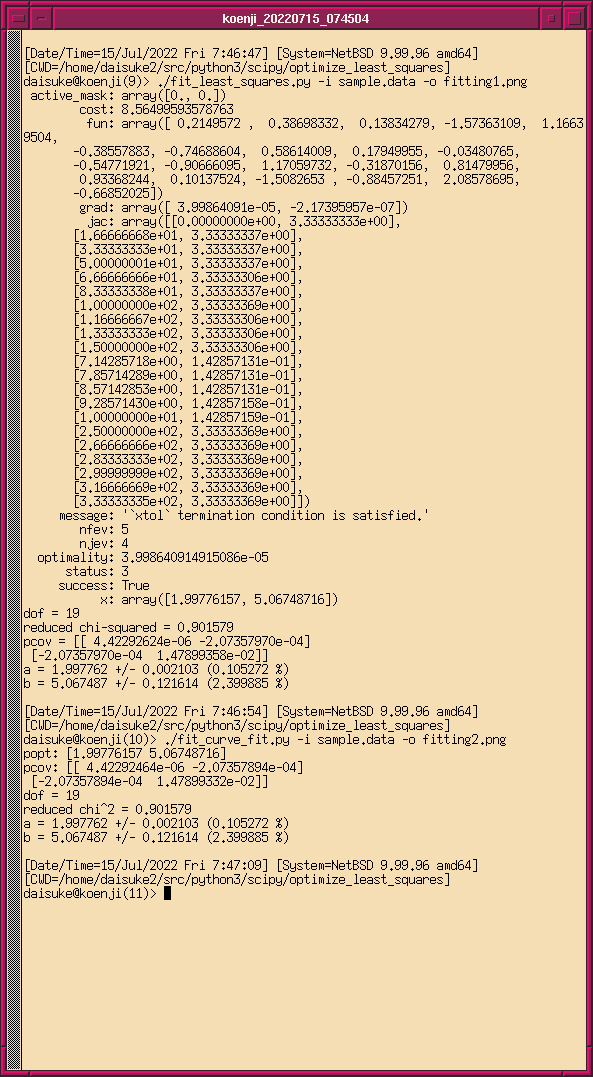
実行結果は以下の通りにござる。 least_squares を使うと、フィッティング により求めた係数の値とヤコビアンが得られるでござる。ヤコビアンから共分 散行列を求めるところは自分で行う必要があるでござる。ヤコビアン J の転 置行列を作り、ヤコビアンの転置行列とヤコビアンの掛け算をし、その逆行列 を作り、 reduced chi-squared を掛ければ、共分散行列が得られるでござる。
% ./fit_least_squares.py -i sample.data -o least_squares.png -r 135
 active_mask: array([0., 0.])
        cost: 8.56499593578763
         fun: array([ 0.2149572 ,  0.38698332,  0.13834279, -1.57363109,  1.16639504,
       -0.38557883, -0.74688604,  0.58614009,  0.17949955, -0.03480765,
       -0.54771921, -0.90666095,  1.17059732, -0.31870156,  0.81479956,
        0.93368244,  0.10137524, -1.5082653 , -0.88457251,  2.08578695,
       -0.66852025])
        grad: array([ 3.99864091e-05, -2.17395957e-07])
         jac: array([[0.00000000e+00, 3.33333333e+00],
       [1.66666668e+01, 3.33333337e+00],
       [3.33333333e+01, 3.33333337e+00],
       [5.00000001e+01, 3.33333337e+00],
       [6.66666666e+01, 3.33333306e+00],
       [8.33333338e+01, 3.33333337e+00],
       [1.00000000e+02, 3.33333369e+00],
       [1.16666667e+02, 3.33333306e+00],
       [1.33333333e+02, 3.33333306e+00],
       [1.50000000e+02, 3.33333306e+00],
       [7.14285718e+00, 1.42857131e-01],
       [7.85714289e+00, 1.42857131e-01],
       [8.57142853e+00, 1.42857131e-01],
       [9.28571430e+00, 1.42857158e-01],
       [1.00000000e+01, 1.42857159e-01],
       [2.50000000e+02, 3.33333369e+00],
       [2.66666666e+02, 3.33333369e+00],
       [2.83333333e+02, 3.33333369e+00],
       [2.99999999e+02, 3.33333369e+00],
       [3.16666669e+02, 3.33333369e+00],
       [3.33333335e+02, 3.33333369e+00]])
     message: '`xtol` termination condition is satisfied.'
        nfev: 5
        njev: 4
  optimality: 3.998640914915086e-05
      status: 3
     success: True
           x: array([1.99776157, 5.06748716])
dof = 19
reduced chi-squared = 0.901579
pcov = [[ 4.42292624e-06 -2.07357970e-04]
 [-2.07357970e-04  1.47899358e-02]]
a = 1.997762 +/- 0.002103 (0.105272 %)
b = 5.067487 +/- 0.121614 (2.399885 %)
|
|---|
|
|---|
|
|---|
そうなってもらわねば困るのでござるが、 curve_fit と least_squares とで 同じ結果が得られたでござる。
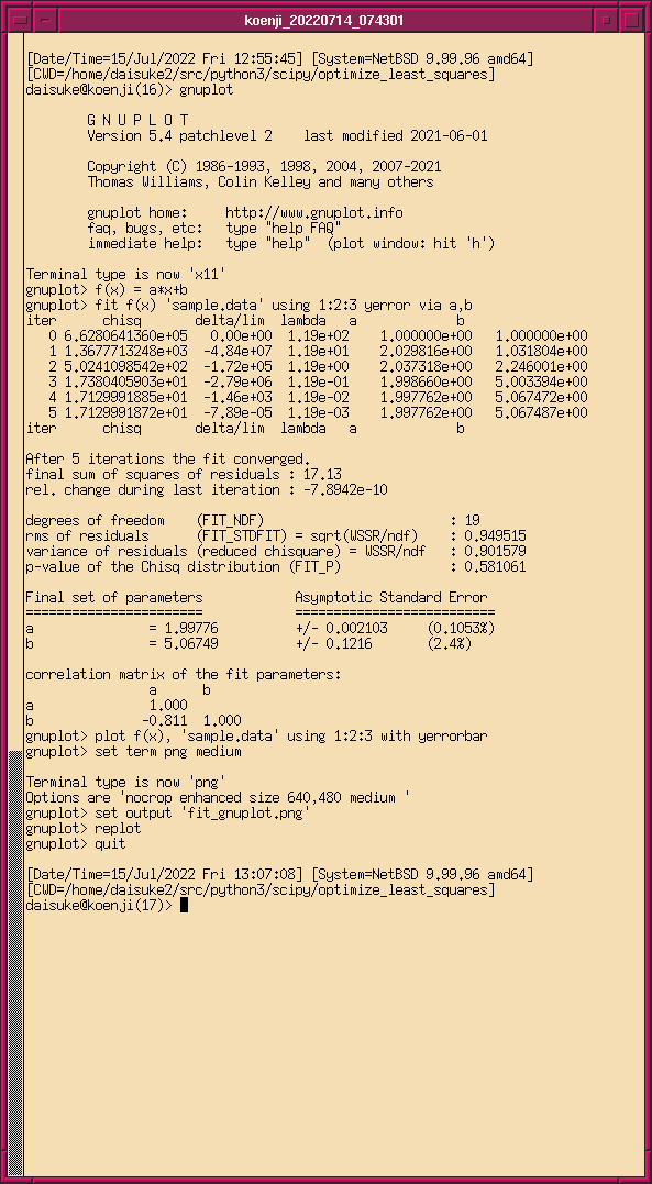
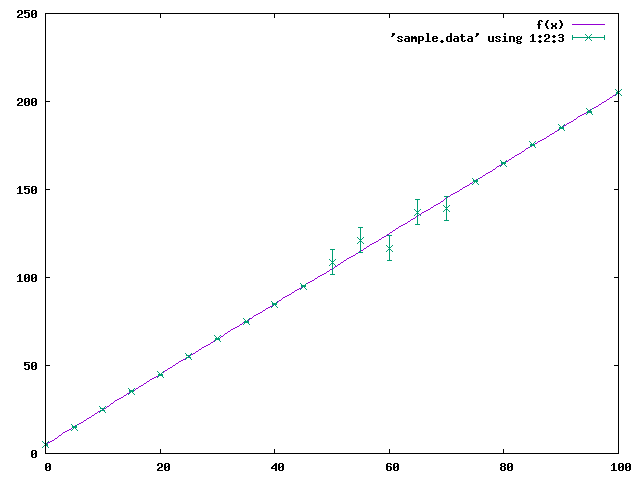
最後に、確認のため、 gnuplot の fit を使って最小二乗法を行ってみるでご ざる。
% gnuplot

        G N U P L O T
        Version 5.4 patchlevel 2    last modified 2021-06-01

        Copyright (C) 1986-1993, 1998, 2004, 2007-2021
        Thomas Williams, Colin Kelley and many others

        gnuplot home:     http://www.gnuplot.info
        faq, bugs, etc:   type "help FAQ"
        immediate help:   type "help"  (plot window: hit 'h')

Terminal type is now 'x11'
gnuplot> f(x) = a*x+b
gnuplot> fit f(x) 'sample.data' using 1:2:3 yerror via a,b
iter      chisq       delta/lim  lambda   a             b
   0 6.6280641360e+05   0.00e+00  1.19e+02    1.000000e+00   1.000000e+00
   1 1.3677713248e+03  -4.84e+07  1.19e+01    2.029816e+00   1.031804e+00
   2 5.0241098542e+02  -1.72e+05  1.19e+00    2.037318e+00   2.246001e+00
   3 1.7380405903e+01  -2.79e+06  1.19e-01    1.998660e+00   5.003394e+00
   4 1.7129991885e+01  -1.46e+03  1.19e-02    1.997762e+00   5.067472e+00
   5 1.7129991872e+01  -7.89e-05  1.19e-03    1.997762e+00   5.067487e+00
iter      chisq       delta/lim  lambda   a             b

After 5 iterations the fit converged.
final sum of squares of residuals : 17.13
rel. change during last iteration : -7.8942e-10

degrees of freedom    (FIT_NDF)                        : 19
rms of residuals      (FIT_STDFIT) = sqrt(WSSR/ndf)    : 0.949515
variance of residuals (reduced chisquare) = WSSR/ndf   : 0.901579
p-value of the Chisq distribution (FIT_P)              : 0.581061

Final set of parameters            Asymptotic Standard Error
=======================            ==========================
a               = 1.99776          +/- 0.002103     (0.1053%)
b               = 5.06749          +/- 0.1216       (2.4%)

correlation matrix of the fit parameters:
                a      b
a               1.000
b              -0.811  1.000
gnuplot> plot f(x), 'sample.data' using 1:2:3 with yerrorbar
gnuplot> set term png medium

Terminal type is now 'png'
Options are 'nocrop enhanced size 640,480 medium '
gnuplot> set output 'fit_gnuplot.png'
gnuplot> replot
gnuplot> quit
|
|---|
|
|---|
gnuplot による結果も curve_fit 及び least_squares と同じになったでござ る。